
Naturgy — Predicción de precio a 24 horas
EDA, feature engineering y XGBoost V1 + V2 sobre electricidad española (2015–2018). Predicción day-ahead del precio del mercado OMIE.

Naturgy Futuro Sostenible
Predicción del precio de la electricidad a 24 horas vista
El reto de negocio
La transición hacia las energías renovables ha introducido una volatilidad extrema en el precio de la electricidad: la solar y la eólica son baratas pero intermitentes, y cuando no producen entran en juego las tecnologías más caras (gas, carbón). Para Naturgy el reto no es solo ser más verde, sino gestionar el riesgo que esa volatilidad introduce en sus márgenes.
La regla de las 12:00 — por qué predecir a 24h
El mercado mayorista español (OMIE) cierra su subasta diaria a las 12:00 del mediodía, fijando los precios de todo el día siguiente. Esto impone una restricción operativa clara: Naturgy necesita saber hoy el precio de mañana. Si la predicción falla, la mesa de trading oferta a ciegas y la comercializadora asume pérdidas al comprar energía cara para cubrir a sus clientes de tarifa fija.
Por eso todo el proyecto se diseña como una predicción day-ahead (t + 24h), usando únicamente información disponible en el momento de predecir (sin data leakage).
Objetivo
Construir una solución capaz de predecir el precio horario de la electricidad con 24 horas de antelación, combinando el histórico del mix energético nacional y las condiciones climáticas de las principales ciudades españolas (2015–2018).
Los datos
Mix energético nacional: generación por tecnología, demanda, previsiones del operador y precio.
Clima de 5 ciudades (Madrid, Barcelona, Sevilla, Valencia, Bilbao): temperatura, viento, humedad, nubosidad, etc.
Qué encontrarás en este notebook
Limpieza y análisis exploratorio de los datos.
Feature engineering con lógica de negocio: clima ponderado por ciudad, vectorización del viento, variables temporales cíclicas, lags y medias móviles.
Entrenamiento y validación de un modelo XGBoost, con todo el año 2018 como test aislado.
INDICE
# Standard library
import warnings

# Third-party libraries
import holidays
import joblib
import matplotlib.pyplot as plt
import numpy as np
import pandas as pd
import seaborn as sns
import xgboost as xgb

from sklearn.compose import ColumnTransformer
from sklearn.metrics import mean_squared_error, mean_absolute_error, r2_score
from sklearn.model_selection import train_test_split
from sklearn.pipeline import Pipeline
from sklearn.preprocessing import StandardScaler

# Local imports
warnings.filterwarnings('ignore')
import viz_utils as viz # funciones de visualización personalizadas para el proyecto
viz.set_naturgy_style()# Comprobración optativa: para gráficas como RTX Laptop 2000 que no son compatibles de forma nativa con xgboost.
import os
print(os.environ.get('LD_LIBRARY_PATH', 'NO DEFINIDA'))NO DEFINIDA
1.2 Paleta de Colores
viz.NORANGE = ['#e37404', '#efaa66', '#f0b983']
viz.NOBLUE  = ['#044474', '#628baa', '#9bb3c4']
Se acceden directamente como viz.NORANGE[0], viz.NOBLUE[0], etc.
viz.show_palette()df_energy = pd.read_parquet('../data/energy_silver.parquet/')
viz.display_dataframe_summary(df_energy, name='Dataset de Energía')
# Se han transpuesto las filas por columnas para una visualización más legible.Dataset de Energía
35,046 filas × 29 columnas | 0 nulos (0.00%) | Tipos: float64: 26, str: 2, datetime64[us]: 1
▸ Primeras 3 filas
| Fila 0 | Fila 1 | Fila 2 | |
|---|---|---|---|
| time | 2014-12-31 23:00:00 | 2015-01-01 00:00:00 | 2015-01-01 01:00:00 |
| generation biomass | 447.00 | 449.00 | 448.00 |
| generation fossil brown coal/lignite | 329.00 | 328.00 | 323.00 |
| generation fossil coal-derived gas | 0.00 | 0.00 | 0.00 |
| generation fossil gas | 4,844.00 | 5,196.00 | 4,857.00 |
| generation fossil hard coal | 4,821.00 | 4,755.00 | 4,581.00 |
| generation fossil oil | 162.00 | 158.00 | 157.00 |
| generation fossil oil shale | 0.00 | 0.00 | 0.00 |
| generation fossil peat | 0.00 | 0.00 | 0.00 |
| generation geothermal | 0.00 | 0.00 | 0.00 |
| generation hydro pumped storage aggregated | Unknown | Unknown | Unknown |
| generation hydro pumped storage consumption | 863.00 | 920.00 | 1,164.00 |
| generation hydro run-of-river and poundage | 1,051.00 | 1,009.00 | 973.00 |
| generation hydro water reservoir | 1,899.00 | 1,658.00 | 1,371.00 |
| generation marine | 0.00 | 0.00 | 0.00 |
| generation nuclear | 7,096.00 | 7,096.00 | 7,099.00 |
| generation other | 43.00 | 43.00 | 43.00 |
| generation other renewable | 73.00 | 71.00 | 73.00 |
| generation solar | 49.00 | 50.00 | 50.00 |
| generation waste | 196.00 | 195.00 | 196.00 |
| generation wind offshore | 0.00 | 0.00 | 0.00 |
| generation wind onshore | 6,378.00 | 5,890.00 | 5,461.00 |
| forecast solar day ahead | 17.00 | 16.00 | 8.00 |
| forecast wind offshore eday ahead | Unknown | Unknown | Unknown |
| forecast wind onshore day ahead | 6,436.00 | 5,856.00 | 5,454.00 |
| total load forecast | 26,118.00 | 24,934.00 | 23,515.00 |
| total load actual | 25,385.00 | 24,382.00 | 22,734.00 |
| price day ahead | 50.10 | 48.10 | 47.33 |
| price actual | 65.41 | 64.92 | 64.48 |
▸ Variables del Dataset (29 columnas)
| Variable | Tipo | No Nulos | Nulos | % Nulos | Ejemplo | |
|---|---|---|---|---|---|---|
| 0 | time | datetime64[us] | 35,046 | 0 | 0.0% | 2014-12-31 23:00:00 |
| 1 | generation biomass | float64 | 35,046 | 0 | 0.0% | 447.00 |
| 2 | generation fossil brown coal/lignite | float64 | 35,046 | 0 | 0.0% | 329.00 |
| 3 | generation fossil coal-derived gas | float64 | 35,046 | 0 | 0.0% | 0.0000 |
| 4 | generation fossil gas | float64 | 35,046 | 0 | 0.0% | 4844.00 |
| 5 | generation fossil hard coal | float64 | 35,046 | 0 | 0.0% | 4821.00 |
| 6 | generation fossil oil | float64 | 35,046 | 0 | 0.0% | 162.00 |
| 7 | generation fossil oil shale | float64 | 35,046 | 0 | 0.0% | 0.0000 |
| 8 | generation fossil peat | float64 | 35,046 | 0 | 0.0% | 0.0000 |
| 9 | generation geothermal | float64 | 35,046 | 0 | 0.0% | 0.0000 |
| 10 | generation hydro pumped storage aggregated | str | 35,046 | 0 | 0.0% | Unknown |
| 11 | generation hydro pumped storage consumption | float64 | 35,046 | 0 | 0.0% | 863.00 |
| 12 | generation hydro run-of-river and poundage | float64 | 35,046 | 0 | 0.0% | 1051.00 |
| 13 | generation hydro water reservoir | float64 | 35,046 | 0 | 0.0% | 1899.00 |
| 14 | generation marine | float64 | 35,046 | 0 | 0.0% | 0.0000 |
| 15 | generation nuclear | float64 | 35,046 | 0 | 0.0% | 7096.00 |
| 16 | generation other | float64 | 35,046 | 0 | 0.0% | 43.00 |
| 17 | generation other renewable | float64 | 35,046 | 0 | 0.0% | 73.00 |
| 18 | generation solar | float64 | 35,046 | 0 | 0.0% | 49.00 |
| 19 | generation waste | float64 | 35,046 | 0 | 0.0% | 196.00 |
| 20 | generation wind offshore | float64 | 35,046 | 0 | 0.0% | 0.0000 |
| 21 | generation wind onshore | float64 | 35,046 | 0 | 0.0% | 6378.00 |
| 22 | forecast solar day ahead | float64 | 35,046 | 0 | 0.0% | 17.00 |
| 23 | forecast wind offshore eday ahead | str | 35,046 | 0 | 0.0% | Unknown |
| 24 | forecast wind onshore day ahead | float64 | 35,046 | 0 | 0.0% | 6436.00 |
| 25 | total load forecast | float64 | 35,046 | 0 | 0.0% | 26118.00 |
| 26 | total load actual | float64 | 35,046 | 0 | 0.0% | 25385.00 |
| 27 | price day ahead | float64 | 35,046 | 0 | 0.0% | 50.10 |
| 28 | price actual | float64 | 35,046 | 0 | 0.0% | 65.41 |
▸ Estadísticas Descriptivas
| N | Media | Std | Min | Q1 | Med | Q3 | Max | |
|---|---|---|---|---|---|---|---|---|
| generation biomass | 35046.00 | 383.51 | 85.35 | 0.00 | 333.00 | 367.00 | 433.00 | 592.00 |
| generation fossil brown coal/lignite | 35046.00 | 448.06 | 354.57 | 0.00 | 0.00 | 509.00 | 757.00 | 999.00 |
| generation fossil coal-derived gas | 35046.00 | 0.00 | 0.00 | 0.00 | 0.00 | 0.00 | 0.00 | 0.00 |
| generation fossil gas | 35046.00 | 5622.74 | 2201.83 | 0.00 | 4126.00 | 4969.00 | 6429.00 | 20034.00 |
| generation fossil hard coal | 35046.00 | 4256.07 | 1961.60 | 0.00 | 2527.00 | 4474.00 | 5838.75 | 8359.00 |
| generation fossil oil | 35046.00 | 298.32 | 52.52 | 0.00 | 263.00 | 300.00 | 330.00 | 449.00 |
| generation fossil oil shale | 35046.00 | 0.00 | 0.00 | 0.00 | 0.00 | 0.00 | 0.00 | 0.00 |
| generation fossil peat | 35046.00 | 0.00 | 0.00 | 0.00 | 0.00 | 0.00 | 0.00 | 0.00 |
| generation geothermal | 35046.00 | 0.00 | 0.00 | 0.00 | 0.00 | 0.00 | 0.00 | 0.00 |
| generation hydro pumped storage consumption | 35046.00 | 475.57 | 792.40 | 0.00 | 0.00 | 68.00 | 616.00 | 4523.00 |
| generation hydro run-of-river and poundage | 35046.00 | 972.11 | 400.77 | 0.00 | 637.00 | 906.00 | 1250.00 | 2000.00 |
| generation hydro water reservoir | 35046.00 | 2605.11 | 1835.20 | 0.00 | 1077.25 | 2164.00 | 3757.00 | 9728.00 |
| generation marine | 35046.00 | 0.00 | 0.00 | 0.00 | 0.00 | 0.00 | 0.00 | 0.00 |
| generation nuclear | 35046.00 | 6263.89 | 839.67 | 0.00 | 5760.00 | 6565.50 | 7025.00 | 7117.00 |
| generation other | 35046.00 | 60.23 | 20.24 | 0.00 | 53.00 | 57.00 | 80.00 | 106.00 |
| generation other renewable | 35046.00 | 85.64 | 14.08 | 0.00 | 73.00 | 88.00 | 97.00 | 119.00 |
| generation solar | 35046.00 | 1432.67 | 1680.12 | 0.00 | 71.00 | 616.00 | 2578.00 | 5792.00 |
| generation waste | 35046.00 | 269.45 | 50.19 | 0.00 | 240.00 | 279.00 | 310.00 | 357.00 |
| generation wind offshore | 35046.00 | 0.00 | 0.00 | 0.00 | 0.00 | 0.00 | 0.00 | 0.00 |
| generation wind onshore | 35046.00 | 5464.48 | 3213.69 | 0.00 | 2933.00 | 4849.00 | 7398.00 | 17436.00 |
| forecast solar day ahead | 35046.00 | 1438.79 | 1677.67 | 0.00 | 69.00 | 576.00 | 2635.00 | 5836.00 |
| forecast wind onshore day ahead | 35046.00 | 5470.68 | 3176.38 | 237.00 | 2979.00 | 4853.00 | 7350.75 | 17430.00 |
| total load forecast | 35046.00 | 28711.26 | 4592.47 | 18105.00 | 24795.00 | 28905.00 | 32263.00 | 41390.00 |
| total load actual | 35046.00 | 28696.37 | 4572.64 | 18041.00 | 24809.25 | 28901.00 | 32187.00 | 41015.00 |
| price day ahead | 35046.00 | 49.87 | 14.62 | 2.06 | 41.49 | 50.52 | 60.53 | 101.99 |
| price actual | 35046.00 | 57.88 | 14.20 | 9.33 | 49.34 | 58.01 | 68.00 | 116.80 |
Hallazgos:
generation hydro pumped storage aggregated y forecast wind offshore eday ahead: se pueden eliminar, su valor en su totalidad es unknown. Probablemente se realizaron mal las agregaciones.
No se observan nulos, por lo que la limpieza inicial del ETL fue robusta. Por otra parte hay variable como: generation fossil coal-derived gas, generation fossil oil shale, etc, que podrían indicar que nunca se llegaron a realizar mediciones sobre ellos o que los sensores no funcionaban (Eliminarlos).
Las energías renovables son las menos estables ya que dependen mucho de las condiciones metereológicas. Por otra parte fuentes de energía como la nuclear son de las más estables.
Elgunas variables son ya predicciones realizadas que nos podrán servir si nuestros modelos consiguen ganar frente a los actuales.
df_weather = pd.read_parquet('../data/weather_features_silver.parquet')
viz.display_dataframe_summary(df_weather, name='Dataset de Clima')
Dataset de Clima
175,271 filas × 15 columnas | 0 nulos (0.00%) | Tipos: float64: 7, int64: 4, str: 3, datetime64[us]: 1
▸ Primeras 3 filas
| Fila 0 | Fila 1 | Fila 2 | |
|---|---|---|---|
| time | 2014-12-31 23:00:00 | 2015-01-01 00:00:00 | 2015-01-01 01:00:00 |
| city_name | Valencia | Valencia | Valencia |
| temp | -2.67 | -2.67 | -3.46 |
| temp_min | -2.67 | -2.67 | -3.46 |
| temp_max | -2.67 | -2.67 | -3.46 |
| pressure | 1,001.00 | 1,001.00 | 1,002.00 |
| humidity | 77.00 | 77.00 | 78.00 |
| wind_speed | 3.60 | 3.60 | 0.00 |
| wind_deg | 62.00 | 62.00 | 23.00 |
| rain_1h | 0.00 | 0.00 | 0.00 |
| rain_3h | 0.00 | 0.00 | 0.00 |
| snow_3h | 0.00 | 0.00 | 0.00 |
| clouds_all | 0.00 | 0.00 | 0.00 |
| weather_main | clear | clear | clear |
| weather_description | sky is clear | sky is clear | sky is clear |
▸ Variables del Dataset (15 columnas)
| Variable | Tipo | No Nulos | Nulos | % Nulos | Ejemplo | |
|---|---|---|---|---|---|---|
| 0 | time | datetime64[us] | 175,271 | 0 | 0.0% | 2014-12-31 23:00:00 |
| 1 | city_name | str | 175,271 | 0 | 0.0% | Valencia |
| 2 | temp | float64 | 175,271 | 0 | 0.0% | -2.67 |
| 3 | temp_min | float64 | 175,271 | 0 | 0.0% | -2.67 |
| 4 | temp_max | float64 | 175,271 | 0 | 0.0% | -2.67 |
| 5 | pressure | int64 | 175,271 | 0 | 0.0% | 1001 |
| 6 | humidity | int64 | 175,271 | 0 | 0.0% | 77 |
| 7 | wind_speed | float64 | 175,271 | 0 | 0.0% | 3.60 |
| 8 | wind_deg | int64 | 175,271 | 0 | 0.0% | 62 |
| 9 | rain_1h | float64 | 175,271 | 0 | 0.0% | 0.0000 |
| 10 | rain_3h | float64 | 175,271 | 0 | 0.0% | 0.0000 |
| 11 | snow_3h | float64 | 175,271 | 0 | 0.0% | 0.0000 |
| 12 | clouds_all | int64 | 175,271 | 0 | 0.0% | 0 |
| 13 | weather_main | str | 175,271 | 0 | 0.0% | clear |
| 14 | weather_description | str | 175,271 | 0 | 0.0% | sky is clear |
▸ Estadísticas Descriptivas
| N | Media | Std | Min | Q1 | Med | Q3 | Max | |
|---|---|---|---|---|---|---|---|---|
| temp | 175271.00 | 16.56 | 8.02 | -10.91 | 10.68 | 16.00 | 22.09 | 42.45 |
| temp_min | 175271.00 | 15.28 | 7.95 | -10.91 | 9.64 | 15.00 | 21.00 | 42.00 |
| temp_max | 175271.00 | 18.02 | 8.61 | -10.91 | 11.78 | 17.00 | 24.00 | 48.00 |
| pressure | 175271.00 | 1016.22 | 12.50 | 918.00 | 1013.00 | 1018.00 | 1022.00 | 1090.00 |
| humidity | 175271.00 | 68.05 | 21.81 | 0.00 | 53.00 | 72.00 | 87.00 | 100.00 |
| wind_speed | 175271.00 | 8.89 | 7.46 | 0.00 | 3.60 | 7.20 | 14.40 | 230.40 |
| wind_deg | 175271.00 | 166.73 | 116.54 | 0.00 | 56.00 | 178.00 | 270.00 | 360.00 |
| rain_1h | 175271.00 | 0.07 | 0.38 | 0.00 | 0.00 | 0.00 | 0.00 | 12.00 |
| rain_3h | 175271.00 | 0.00 | 0.01 | 0.00 | 0.00 | 0.00 | 0.00 | 2.31 |
| snow_3h | 175271.00 | 0.00 | 0.22 | 0.00 | 0.00 | 0.00 | 0.00 | 21.50 |
| clouds_all | 175271.00 | 24.34 | 30.34 | 0.00 | 0.00 | 16.00 | 40.00 | 100.00 |
viz.show_unique_values(df_weather, name='Dataset de Clima')▸ Variables de Texto (3 columnas)
city_name (5 valores únicos)
weather_main (12 valores únicos)
weather_description (41 valores únicos)
Hallazgos:
Tanto rain3h como snow 3h son candidatos a eliminarse. Su media es de 0.00 aportando ruido a los modelos.
temp_min/max no hace referencia a la diferencia entre las temperaturas a lo largo de esa hora sino que representan distintas estaciones de mediciones de temperatura de la misma ciudad. El referente real de temeperatura será temp, los otros probablemente eliminarlos debido a una alta correlación entre ellas.
Los datos son 5 veces a los de generación. Ésto se debe a que pertenecen a 5 ciudades disintas de España. Habría que pensar si darle pesos distintos dependiendo de la ciudad (en Madrid se consume mucha más electricidad que en bilbao o que en Valencia).
weather_description es la versión extendida de weather_main por así decirlo, nos mantenemos solo con el último ya que prácticamente están aportando lo mismo y 41 features más para el modelo puede ser un poco contraproducente.
2.1.1 Eliminación de variables irrelevantes
En los años de este dataset (2015-2018), la red eléctrica española no tenía instaladas estas tecnologías a nivel comercial: generation wind offshore, forecast wind offshore eday ahead, generation geothermal, generation marine, generation fossil coal-derived gas, oil shale, peat.
cols_to_drop_energy = [
    'generation hydro pumped storage aggregated',
    'forecast wind offshore eday ahead',
    'generation fossil coal-derived gas',
    'generation fossil oil shale',
    'generation fossil peat',
    'generation geothermal',
    'generation marine',
    'generation wind offshore',
    'price day ahead',

    # Producen data leakage
    'generation biomass',
    'generation fossil brown coal/lignite',
    'generation fossil gas',
    'generation fossil hard coal',
    'generation fossil oil',
    'generation hydro run-of-river and poundage',
    'generation hydro water reservoir',
    'generation nuclear',
    'generation other',
    'generation other renewable',
    'generation solar',
    'generation waste',
    'generation wind onshore'
]

df_energy_clean = df_energy.drop(columns=cols_to_drop_energy, errors='ignore')

print(f"Dataset original: {df_energy.shape[1]} columnas")
print(f"Dataset limpio:   {df_energy_clean.shape[1]} columnas")
Dataset original: 29 columnas Dataset limpio: 7 columnas
2.2.1 Eliminación de weather_description
Eliminamos weather_description (41 categorías) porque es redundante con weather_main y añadiría ruido innecesario al modelo. La información meteorológica ya queda suficientemente capturada por las macro-categorías de weather_main y las variables numéricas (temp, humidity, clouds_all).
print(f"Columnas en clima antes: {df_weather.shape[1]}")
df_weather = df_weather.drop(columns=["weather_description"])
print(f"Columnas en clima después: {df_weather.shape[1]}")
print("Columna 'weather_description' eliminada correctamente.")
Columnas en clima antes: 15 Columnas en clima después: 14 Columna 'weather_description' eliminada correctamente.
2.2.2 Vectorización del viento
La naturaleza del viento es vectorial, por lo que intentar sumar las velocidades como si fuesen escalares sería incorrecto y no representaría el mundo real.
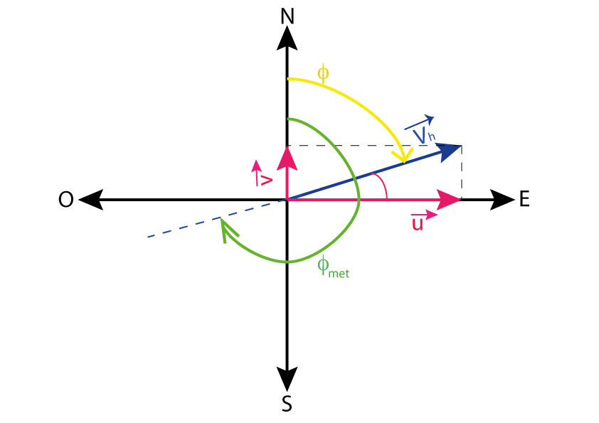
Como el dataset de energía es a nivel nacional, intentaremos hacer la media de las condiciones del clima, que son por ciudad. Aunque perdamos algo de información, al calcular a nivel nacional no nos afectará tanto.
numeric_cols_weather = df_weather.select_dtypes(include=np.number).columns

# Conversión a componente vectorial del viento (componente este-oeste)
df_weather['wind_x'] = df_weather['wind_speed'] * np.cos(np.radians((90 - df_weather['wind_deg']) % 360))
' barcelona' vs 'barcelona': en el dataset se aprecia un espacio inicial en algunos nombres de ciudad. Esto puede provocar errores al tratar el dataset, así que lo normalizamos.
df_weather['city_name'] = df_weather['city_name'].str.strip()2.2.3 Reducción de cardinalidad y One-Hot Encoding
En weather_main hay algunas categorías como fog, haze o smoke que ocurren muy pocas veces. Para evitar que produzcan ruido las agruparemos en macro-categorías, de forma que el modelo pueda aprender patrones de forma más eficiente.
weather_mapping = {
    'clear': 'Clear',
    'clouds': 'Cloudy',
    'rain': 'Rain',
    'drizzle': 'Rain',
    'thunderstorm': 'Storm',
    'snow': 'Snow',
    'squall': 'Wind',  # Ráfagas de viento como categoría separada
    'mist': 'Visibility_Issues',
    'fog': 'Visibility_Issues',
    'haze': 'Visibility_Issues',
    'smoke': 'Visibility_Issues',
    'dust': 'Visibility_Issues'
}

df_weather["weather_grouped"] = df_weather["weather_main"].str.lower().replace(weather_mapping)

#  One-Hot Encoding
clima_dummies = pd.get_dummies(df_weather["weather_grouped"], prefix="weather")

# Unión al dataset original
df_weather = pd.concat([df_weather, clima_dummies], axis=1)
2.2.4 Agregación ponderada por ciudad
Si lo pensamos detalladamente, no todas las ciudades tienen la misma demanda energética. Si en Madrid hace calor, la demanda se dispara mucho más que en Bilbao o Valencia. Añadimos pesos a cada ciudad para que el promedio nacional sea más fiel a la lógica de negocio.
pesos_ciudades = {
    'Madrid': 0.28,
    'Barcelona': 0.28,
    'Seville': 0.18,
    'Valencia': 0.16,
    'Bilbao': 0.10
}
df_weather["peso"] = df_weather["city_name"].map(pesos_ciudades)

columnas_numericas = [
    'temp', 'humidity', 'pressure', 'wind_speed', 'wind_x',
    'clouds_all', 'rain_1h',
    'weather_Clear', 'weather_Cloudy', 'weather_Rain', 'weather_Storm',
    'weather_Visibility_Issues', 'weather_Snow', 'weather_Wind'
]


columnas_existentes = [col for col in columnas_numericas if col in df_weather.columns]

def promedio_ponderado(df_group):
    weights = df_group["peso"].values
    result = {}
    for col in columnas_existentes:
        result[col] = np.average(df_group[col], weights=weights)
    return pd.Series(result)

# Agrupación final: 1 fila por timestamp
df_weather_nacional = df_weather.groupby("time").apply(promedio_ponderado).reset_index()viz.display_describe(df_weather_nacional, name="Clima Nacional Ponderado")Estadísticas Descriptivas — Clima Nacional Ponderado
14 variables numéricas | 35,064 registros
| N | Media | Std | Min | Q1 | Med | Q3 | Max | |
|---|---|---|---|---|---|---|---|---|
| temp | 35,064.00 | 16.67 | 7.44 | -1.47 | 10.93 | 15.92 | 22.23 | 36.61 |
| humidity | 35,064.00 | 66.91 | 15.66 | 19.86 | 54.88 | 68.12 | 79.56 | 100.00 |
| pressure | 35,064.00 | 1,015.77 | 8.88 | 974.78 | 1,012.60 | 1,016.78 | 1,020.82 | 1,039.84 |
| wind_speed | 35,064.00 | 9.12 | 4.92 | 0.00 | 5.62 | 8.06 | 11.59 | 54.29 |
| wind_x | 35,064.00 | -1.45 | 5.51 | -44.96 | -3.51 | -0.96 | 1.54 | 22.51 |
| clouds_all | 35,064.00 | 22.36 | 17.86 | 0.00 | 8.20 | 17.60 | 33.10 | 94.24 |
| rain_1h | 35,064.00 | 0.07 | 0.22 | 0.00 | 0.00 | 0.00 | 0.03 | 4.29 |
| weather_Clear | 35,064.00 | 0.50 | 0.31 | 0.00 | 0.26 | 0.46 | 0.74 | 1.00 |
| weather_Cloudy | 35,064.00 | 0.38 | 0.27 | 0.00 | 0.16 | 0.38 | 0.54 | 1.00 |
| weather_Rain | 35,064.00 | 0.09 | 0.17 | 0.00 | 0.00 | 0.00 | 0.10 | 1.00 |
| weather_Storm | 35,064.00 | 0.00 | 0.03 | 0.00 | 0.00 | 0.00 | 0.00 | 0.74 |
| weather_Visibility_Issues | 35,064.00 | 0.03 | 0.08 | 0.00 | 0.00 | 0.00 | 0.00 | 0.84 |
| weather_Snow | 35,064.00 | 0.00 | 0.01 | 0.00 | 0.00 | 0.00 | 0.00 | 0.38 |
| weather_Wind | 35,064.00 | 0.00 | 0.00 | 0.00 | 0.00 | 0.00 | 0.00 | 0.18 |
print("Resumen")
print(f"Dataset de energía:  {df_energy_clean.shape}")
print(f"Dataset de clima:    {df_weather_nacional.shape}")

print(f"Rango temporal energía: {df_energy_clean['time'].min()} -> {df_energy_clean['time'].max()}")
print(f"Rango temporal clima:    {df_weather_nacional['time'].min()} -> {df_weather_nacional['time'].max()}")

print(f"Columnas energía: {list(df_energy_clean.columns)}")
print(f"Columnas clima: {list(df_weather_nacional.columns)}")
Resumen Dataset de energía: (35046, 7) Dataset de clima: (35064, 15) Rango temporal energía: 2014-12-31 23:00:00 -> 2018-12-31 22:00:00 Rango temporal clima: 2014-12-31 23:00:00 -> 2018-12-31 22:00:00 Columnas energía: ['time', 'generation hydro pumped storage consumption', 'forecast solar day ahead', 'forecast wind onshore day ahead', 'total load forecast', 'total load actual', 'price actual'] Columnas clima: ['time', 'temp', 'humidity', 'pressure', 'wind_speed', 'wind_x', 'clouds_all', 'rain_1h', 'weather_Clear', 'weather_Cloudy', 'weather_Rain', 'weather_Storm', 'weather_Visibility_Issues', 'weather_Snow', 'weather_Wind']
Sorprendentemente hay una discrepancia en la cantidad de datos entre ambos datasets. Si calculamos las horas del intervalo temporal de los datos: - (365 días × 3 años) + (366 días × 1 año) = 1.461 días en total. - 1.461 días × 24 horas = 35.064 horas exactas.
Es decir, le faltan datos al dataset de energía.
Para solucionarlo propongo rellenar los datos faltantes con interpolación lineal (Recomendado por gemini, hay que comprobar que tenga sentido). Es la forma más simple de estimar los huecos. No obstante, antes comprobaré que no haya saltos faltantes > 3h.
df_energy['time'] = pd.to_datetime(df_energy['time'])

# Filas donde el salto con la anterior sea mayor de 1 hora
saltos_temporales = df_energy[df_energy['time'].diff() > pd.Timedelta(hours=1)]

print(saltos_temporales['time'])
99 2015-01-05 03:00:00 107 2015-01-05 17:00:00 444 2015-01-19 20:00:00 634 2015-01-27 19:00:00 651 2015-01-28 13:00:00 2517 2015-04-16 08:00:00 2696 2015-04-23 20:00:00 3955 2015-06-15 08:00:00 6572 2015-10-02 10:00:00 8034 2015-12-02 09:00:00 13325 2016-07-09 21:00:00 30879 2018-07-11 08:00:00 Name: time, dtype: datetime64[us]
df_master = pd.merge(df_weather_nacional, df_energy_clean, on='time', how='outer')

df_master = df_master.sort_values('time').reset_index(drop=True)

print("Nulos antes de interpolar:")
print(df_master.isnull().sum()[df_master.isnull().sum() > 0])

# Interpolación lineal
columnas_a_interpolar = df_master.select_dtypes(include=[np.number]).columns
df_master[columnas_a_interpolar] = df_master[columnas_a_interpolar].interpolate(method='linear')

print("\nTabla final")
print(f"Filas totales: {df_master.shape[0]}")
print(f"Nulos restantes en el dataset: {df_master.isnull().sum().sum()}")
Nulos antes de interpolar: generation hydro pumped storage consumption 18 forecast solar day ahead 18 forecast wind onshore day ahead 18 total load forecast 18 total load actual 18 price actual 18 dtype: int64 Tabla final Filas totales: 35064 Nulos restantes en el dataset: 0
viz.display_dataframe_summary(df_master, name='Dataset Maestro')Dataset Maestro
35,064 filas × 21 columnas | 0 nulos (0.00%) | Tipos: float64: 20, datetime64[us]: 1
▸ Primeras 3 filas
| Fila 0 | Fila 1 | Fila 2 | |
|---|---|---|---|
| time | 2014-12-31 23:00:00 | 2015-01-01 00:00:00 | 2015-01-01 01:00:00 |
| temp | 0.01 | 0.02 | -0.45 |
| humidity | 81.16 | 81.16 | 80.88 |
| pressure | 1,012.46 | 1,012.36 | 1,012.90 |
| wind_speed | 9.29 | 9.29 | 10.37 |
| wind_x | 5.94 | 5.94 | 4.87 |
| clouds_all | 0.00 | 0.00 | 0.00 |
| rain_1h | 0.00 | 0.00 | 0.00 |
| weather_Clear | 1.00 | 1.00 | 1.00 |
| weather_Cloudy | 0.00 | 0.00 | 0.00 |
| weather_Rain | 0.00 | 0.00 | 0.00 |
| weather_Storm | 0.00 | 0.00 | 0.00 |
| weather_Visibility_Issues | 0.00 | 0.00 | 0.00 |
| weather_Snow | 0.00 | 0.00 | 0.00 |
| weather_Wind | 0.00 | 0.00 | 0.00 |
| generation hydro pumped storage consumption | 863.00 | 920.00 | 1,164.00 |
| forecast solar day ahead | 17.00 | 16.00 | 8.00 |
| forecast wind onshore day ahead | 6,436.00 | 5,856.00 | 5,454.00 |
| total load forecast | 26,118.00 | 24,934.00 | 23,515.00 |
| total load actual | 25,385.00 | 24,382.00 | 22,734.00 |
| price actual | 65.41 | 64.92 | 64.48 |
▸ Variables del Dataset (21 columnas)
| Variable | Tipo | No Nulos | Nulos | % Nulos | Ejemplo | |
|---|---|---|---|---|---|---|
| 0 | time | datetime64[us] | 35,064 | 0 | 0.0% | 2014-12-31 23:00:00 |
| 1 | temp | float64 | 35,064 | 0 | 0.0% | 0.0052 |
| 2 | humidity | float64 | 35,064 | 0 | 0.0% | 81.16 |
| 3 | pressure | float64 | 35,064 | 0 | 0.0% | 1012.46 |
| 4 | wind_speed | float64 | 35,064 | 0 | 0.0% | 9.29 |
| 5 | wind_x | float64 | 35,064 | 0 | 0.0% | 5.94 |
| 6 | clouds_all | float64 | 35,064 | 0 | 0.0% | 0.0000 |
| 7 | rain_1h | float64 | 35,064 | 0 | 0.0% | 0.0000 |
| 8 | weather_Clear | float64 | 35,064 | 0 | 0.0% | 1.00 |
| 9 | weather_Cloudy | float64 | 35,064 | 0 | 0.0% | 0.0000 |
| 10 | weather_Rain | float64 | 35,064 | 0 | 0.0% | 0.0000 |
| 11 | weather_Storm | float64 | 35,064 | 0 | 0.0% | 0.0000 |
| 12 | weather_Visibility_Issues | float64 | 35,064 | 0 | 0.0% | 0.0000 |
| 13 | weather_Snow | float64 | 35,064 | 0 | 0.0% | 0.0000 |
| 14 | weather_Wind | float64 | 35,064 | 0 | 0.0% | 0.0000 |
| 15 | generation hydro pumped storage consumption | float64 | 35,064 | 0 | 0.0% | 863.00 |
| 16 | forecast solar day ahead | float64 | 35,064 | 0 | 0.0% | 17.00 |
| 17 | forecast wind onshore day ahead | float64 | 35,064 | 0 | 0.0% | 6436.00 |
| 18 | total load forecast | float64 | 35,064 | 0 | 0.0% | 26118.00 |
| 19 | total load actual | float64 | 35,064 | 0 | 0.0% | 25385.00 |
| 20 | price actual | float64 | 35,064 | 0 | 0.0% | 65.41 |
▸ Estadísticas Descriptivas
| N | Media | Std | Min | Q1 | Med | Q3 | Max | |
|---|---|---|---|---|---|---|---|---|
| temp | 35064.00 | 16.67 | 7.44 | -1.47 | 10.93 | 15.92 | 22.23 | 36.61 |
| humidity | 35064.00 | 66.91 | 15.66 | 19.86 | 54.88 | 68.12 | 79.56 | 100.00 |
| pressure | 35064.00 | 1015.77 | 8.88 | 974.78 | 1012.60 | 1016.78 | 1020.82 | 1039.84 |
| wind_speed | 35064.00 | 9.12 | 4.92 | 0.00 | 5.62 | 8.06 | 11.59 | 54.29 |
| wind_x | 35064.00 | -1.45 | 5.51 | -44.96 | -3.51 | -0.96 | 1.54 | 22.51 |
| clouds_all | 35064.00 | 22.36 | 17.86 | 0.00 | 8.20 | 17.60 | 33.10 | 94.24 |
| rain_1h | 35064.00 | 0.07 | 0.22 | 0.00 | 0.00 | 0.00 | 0.03 | 4.29 |
| weather_Clear | 35064.00 | 0.50 | 0.31 | 0.00 | 0.26 | 0.46 | 0.74 | 1.00 |
| weather_Cloudy | 35064.00 | 0.38 | 0.27 | 0.00 | 0.16 | 0.38 | 0.54 | 1.00 |
| weather_Rain | 35064.00 | 0.09 | 0.17 | 0.00 | 0.00 | 0.00 | 0.10 | 1.00 |
| weather_Storm | 35064.00 | 0.00 | 0.03 | 0.00 | 0.00 | 0.00 | 0.00 | 0.74 |
| weather_Visibility_Issues | 35064.00 | 0.03 | 0.08 | 0.00 | 0.00 | 0.00 | 0.00 | 0.84 |
| weather_Snow | 35064.00 | 0.00 | 0.01 | 0.00 | 0.00 | 0.00 | 0.00 | 0.38 |
| weather_Wind | 35064.00 | 0.00 | 0.00 | 0.00 | 0.00 | 0.00 | 0.00 | 0.18 |
| generation hydro pumped storage consumption | 35064.00 | 475.58 | 792.31 | 0.00 | 0.00 | 68.00 | 616.00 | 4523.00 |
| forecast solar day ahead | 35064.00 | 1438.92 | 1677.49 | 0.00 | 69.00 | 576.00 | 2636.00 | 5836.00 |
| forecast wind onshore day ahead | 35064.00 | 5471.15 | 3176.24 | 237.00 | 2979.00 | 4855.00 | 7353.00 | 17430.00 |
| total load forecast | 35064.00 | 28711.85 | 4593.98 | 18105.00 | 24793.75 | 28906.00 | 32263.25 | 41390.00 |
| total load actual | 35064.00 | 28697.00 | 4573.80 | 18041.00 | 24808.75 | 28901.00 | 32189.25 | 41015.00 |
| price actual | 35064.00 | 57.89 | 14.21 | 9.33 | 49.35 | 58.02 | 68.01 | 116.80 |
viz.plot_target_correlation(df_master, target_col='price actual', figsize=(6, 8))
(<Figure size 600x800 with 2 Axes>,
 <Axes: title={'center': 'Correlación de Variables vs price actual'}>)
En un principio tenía pensado eliminar hydro pumped consumption, lo que hubiera sido un gran error ya que aporta mucha información al modelo. Por otra parte, el resto tiene bastante sentido: las generaciones de carbón y fósiles son las más caras, mientras que las renovables son mucho más baratas.
Es curioso ver cómo se refleja el mercado eléctrico: si algo abarata el precio, arrastra al resto y viceversa. Es como una competencia feroz entre las distintas fuentes de generación de energía.
viz.plot_target_scatter(
    df_master,
    target_col='price actual',
    n_cols=3,
    figsize=(18, None),
    alpha=0.1
)
(<Figure size 1800x3150 with 21 Axes>,
 array([<Axes: title={'center': 'temp\n(r = +0.08)'}, ylabel='price actual'>,
        <Axes: title={'center': 'humidity\n(r = -0.05)'}>,
        <Axes: title={'center': 'pressure\n(r = +0.12)'}>,
        <Axes: title={'center': 'wind_speed\n(r = -0.24)'}, ylabel='price actual'>,
        <Axes: title={'center': 'wind_x\n(r = +0.22)'}>,
        <Axes: title={'center': 'clouds_all\n(r = -0.09)'}>,
        <Axes: title={'center': 'rain_1h\n(r = -0.07)'}, ylabel='price actual'>,
        <Axes: title={'center': 'weather_Clear\n(r = +0.10)'}>,
        <Axes: title={'center': 'weather_Cloudy\n(r = -0.08)'}>,
        <Axes: title={'center': 'weather_Rain\n(r = -0.09)'}, ylabel='price actual'>,
        <Axes: title={'center': 'weather_Storm\n(r = +0.04)'}>,
        <Axes: title={'center': 'weather_Visibility_Issues\n(r = +0.05)'}>,
        <Axes: title={'center': 'weather_Snow\n(r = +0.01)'}, ylabel='price actual'>,
        <Axes: title={'center': 'weather_Wind\n(r = +0.00)'}>,
        <Axes: title={'center': 'generation hydro pumped storage consumption\n(r = -0.43)'}>,
        <Axes: title={'center': 'forecast solar day ahead\n(r = +0.10)'}, ylabel='price actual'>,
        <Axes: title={'center': 'forecast wind onshore day ahead\n(r = -0.22)'}>,
        <Axes: title={'center': 'total load forecast\n(r = +0.44)'}>,
        <Axes: title={'center': 'total load actual\n(r = +0.44)'}, ylabel='price actual'>,
        <Axes: >, <Axes: >], dtype=object))
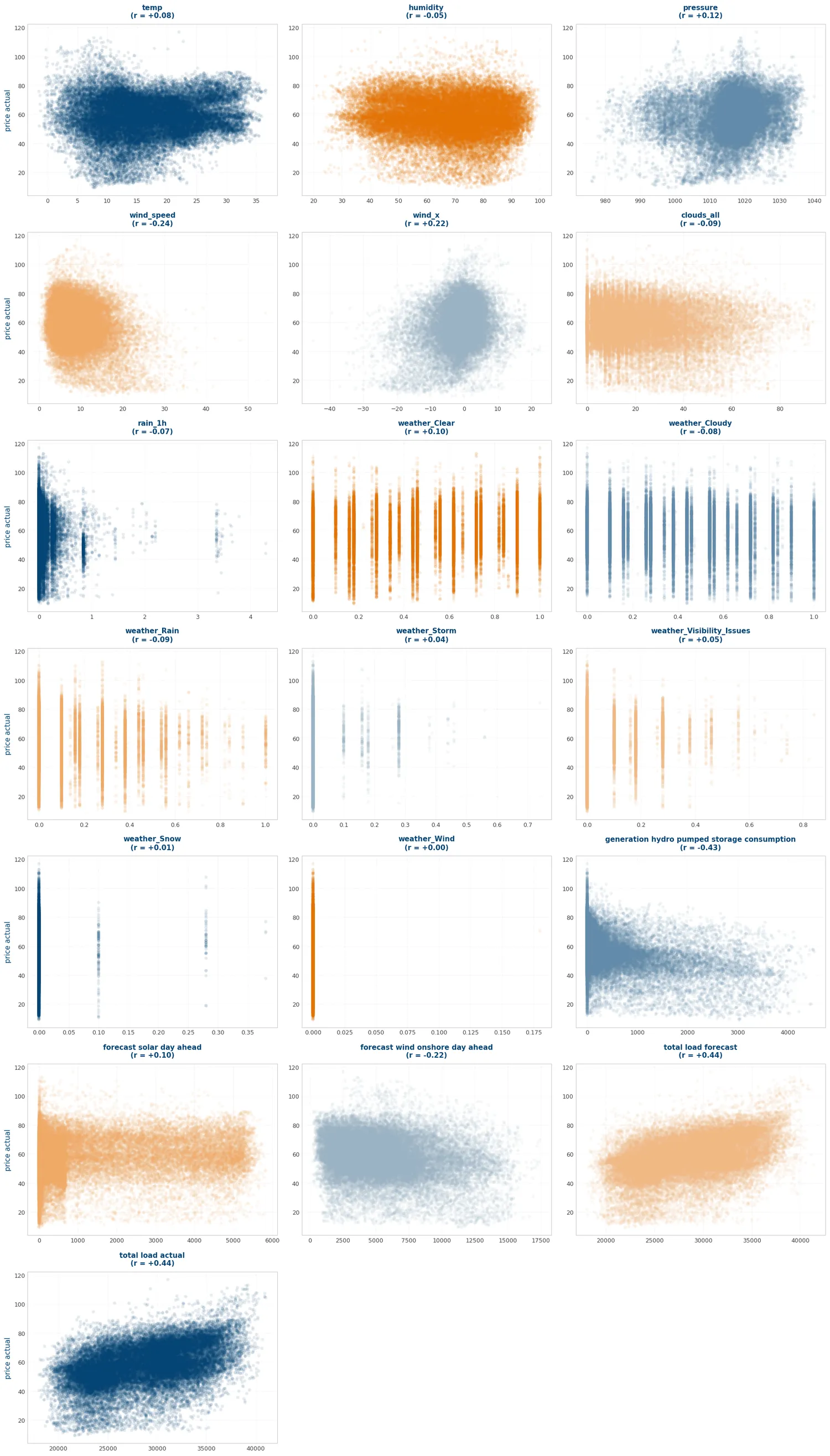
Podemos apreciar que hay variables que generan ruido al modelo, ya que no se aprecian patrones que pueda aprovechar: wind_y es literalmente una nube sin forma y con una correlación muy baja. Por otra parte, wind_x se salva porque sí se aprecia una ligera tendencia que el modelo podría captar. Otras como weather_Visibility_Issues no aportan nada: se ven prácticamente igual en cada segmento. Lo mismo ocurre con más variables.
viz.plot_target_boxplot_by_time(
    df_master,
    time_col='time',
    target_col='price actual',
    figsize=(10, 5),
    title="Distribución del precio de la Luz por hora del día",
    show_stats=True
)
(<Figure size 1000x500 with 1 Axes>,
 <Axes: title={'center': 'Distribución del precio de la Luz por hora del día'}, xlabel='Hora del Día (0-23)', ylabel='price actual'>)
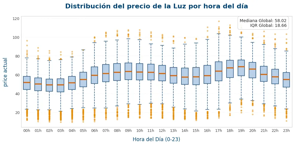
Esto era para comprobar que efectivamente el precio de la luz sigue un patrón cíclico: en las horas de madrugada hay menos demanda y luego, en horas pico como las 9:00 o las 19:00, el precio sube bastante.
cols_legales = [
    'temp', 'humidity', 'pressure', 'wind_speed', 'clouds_all',
    'total load forecast', 'forecast solar day ahead', 'forecast wind onshore day ahead',
    'price actual'
]

viz.plot_correlation_heatmap(
    df_master,
    columns=cols_legales,
    figsize=(12, 10),
    title="Correlación entre predictores legales y precio"
)
(<Figure size 1200x1000 with 2 Axes>,
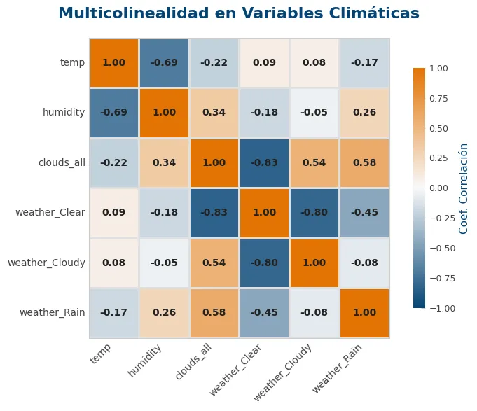
<Axes: title={'center': 'Correlación entre predictores legales y precio'}>)cols_clima = ['temp', 'humidity', 'clouds_all', 'weather_Clear', 'weather_Cloudy', 'weather_Rain']
viz.plot_correlation_heatmap(
df_master,
columns=cols_clima,
figsize=(8, 6),
title="Multicolinealidad en Variables Climáticas"
)
(<Figure size 800x600 with 2 Axes>,
 <Axes: title={'center': 'Multicolinealidad en Variables Climáticas'}>)
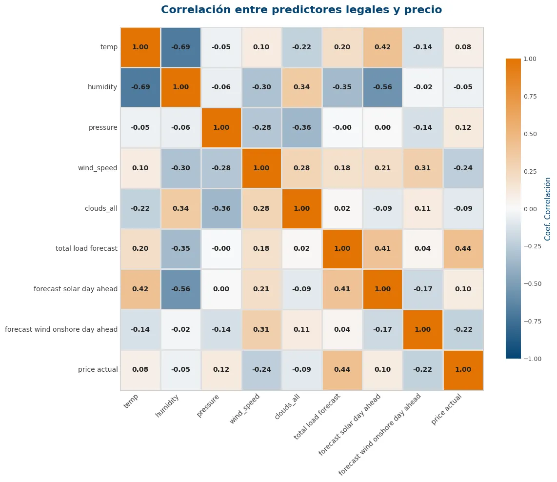
Se aprecian correlaciones muy fuertes entre clouds_all y weather_Clear, y entre weather_Cloudy y weather_Clear. Como clouds_all es numérica y las otras dos son binarias, la primera explicará muchísimo mejor cuántas nubes hay.
Dado que tenemos correlaciones no lineales y no conozco algoritmos más complejos de ML, me he decantado por usar XGBoost y, si hay tiempo, una MLP simple. Esto último implicaría añadir más pasos en este apartado y no supondría necesariamente mejores resultados.
En principio no usaré VIF ni tratamiento de outliers, ya que XGBoost los soporta bien.
columnas_a_borrar = [
    'weather_Wind',
    # 'wind_x',
    'weather_Snow',
    'weather_Storm',
    'weather_Visibility_Issues',
    'weather_Clear',
    'weather_Cloudy'
]

df_master = df_master.drop(columns=columnas_a_borrar)
5.2 Creación de características temporales (festivos y cíclicas)
Creamos características temporales y transformamos las cíclicas en componentes de seno y coseno para capturar la naturaleza periódica de los datos temporales.
# Protección contra el KeyError: si 'time' sigue siendo columna, la pasamos a índice.
if 'time' in df_master.columns:
    df_master = df_master.set_index('time')

# Índice como fecha sin zona horaria (para que cuadre con los festivos)
df_master.index = pd.to_datetime(df_master.index, utc=True).tz_localize(None)

es_holidays = holidays.Spain(years=range(2015, 2020))
festivos_dt = pd.to_datetime(sorted(es_holidays.keys()))

# festivo?
df_master['is_holiday'] = df_master.index.normalize().isin(festivos_dt).astype(int)

# Es víspera de festivo?
visperas = festivos_dt - pd.Timedelta(days=1)
df_master['is_holiday_eve'] = df_master.index.normalize().isin(visperas).astype(int)

# Feature numérica: días hasta/desde el festivo
fechas_actuales = df_master.index.normalize()

def calc_days_to(fecha):
    diffs = (festivos_dt - fecha).days
    futuros = diffs[diffs >= 0]
    return futuros.min() if len(futuros) > 0 else 0

def calc_days_from(fecha):
    diffs = (fecha - festivos_dt).days
    pasados = diffs[diffs >= 0]
    return pasados.min() if len(pasados) > 0 else 0

df_master['days_to_holiday'] = fechas_actuales.map(calc_days_to)
df_master['days_from_holiday'] = fechas_actuales.map(calc_days_from)

print(f"Festivos cargados: {len(festivos_dt)}")
print(f"Registros en festivo: {df_master['is_holiday'].sum()}")
print(f"Registros en víspera: {df_master['is_holiday_eve'].sum()}")
Festivos cargados: 43 Registros en festivo: 840 Registros en víspera: 840
# Extracción de componentes temporales
df_master['hour'] = df_master.index.hour
df_master['dayofweek'] = df_master.index.dayofweek
df_master['month'] = df_master.index.month
df_master['dayofyear'] = df_master.index.dayofyear

# Transformaciones cíclicas
ciclos = {
    'hour': 24,
    'dayofweek': 7,
    'month': 12
}

for col, periodo in ciclos.items():
    df_master[f'{col}_sin'] = np.sin(2 * np.pi * df_master[col] / periodo)
    df_master[f'{col}_cos'] = np.cos(2 * np.pi * df_master[col] / periodo)

# Borrado de las columnas temporales
df_master = df_master.drop(columns=['hour', 'dayofweek', 'month', 'dayofyear'])
5.3 Medias móviles y volatilidad
Para modelos de predicción a futuro, lo ideal es que el conjunto de datos responda a preguntas tan simples como: ¿qué fue lo último que pasó hace una hora?, ¿cómo era la tendencia hace 24h?, etc. Siguiendo esta lógica podemos aprovechar dos estrategias fundamentales (medias móviles y desviaciones), de forma que capturaremos información bastante interesante de estas series temporales.
# TENDENCIA: Media móvil de 24 horas y 168 horas (desplazadas 1h)
df_master['price_roll_mean_24h'] = df_master['price actual'].shift(1).rolling(window=24).mean()
df_master['price_roll_mean_168h'] = df_master['price actual'].shift(1).rolling(window=168).mean()

# VOLATILIDAD: Desviación estándar de las últimas 24 horas (desplazada 1h)
df_master['price_roll_std_24h'] = df_master['price actual'].shift(1).rolling(window=24).std()

# EXTREMOS: Máximos y mínimos recientes (desplazados 1h)
df_master['price_roll_max_24h'] = df_master['price actual'].shift(1).rolling(window=24).max()
df_master['price_roll_min_24h'] = df_master['price actual'].shift(1).rolling(window=24).min()

df_master = df_master.dropna()
5.4 Lags
Es el valor de la misma variable en un período anterior (t-n). Me recuerda un poco al lag de los videojuegos.
lags_clave = [1, 24, 168]

def add_lags(df, col, lags):
    for lag in lags:
        df[f'{col}_lag_{lag}h'] = df[col].shift(lag)
    return df

df_master = add_lags(df_master, 'price actual', lags_clave)
df_master = add_lags(df_master, 'total load actual', lags_clave)

df_master = df_master.dropna()

print(f"Dimensiones: {df_master.shape}")
Dimensiones: (34728, 35)
esta_ordenado = df_master.index.is_monotonic_increasing

diferencia_tiempo = df_master.index.to_series().diff().dropna().value_counts()

print(f"¿Está el índice ordenado cronológicamente?: {esta_ordenado}")
print("Frecuencia de los saltos de tiempo:")
print(diferencia_tiempo)
¿Está el índice ordenado cronológicamente?: True Frecuencia de los saltos de tiempo: time 0 days 01:00:00 34727 Name: count, dtype: int64
viz.display_dataframe_summary(df_master, name='Dataset Maestro (tras Feature Engineering)')Dataset Maestro (tras Feature Engineering)
34,728 filas × 35 columnas | 0 nulos (0.00%) | Tipos: float64: 31, int64: 4
▸ Primeras 3 filas
| Fila 0 | Fila 1 | Fila 2 | |
|---|---|---|---|
| temp | 6.39 | 6.44 | 6.42 |
| humidity | 77.50 | 75.64 | 74.42 |
| pressure | 1,006.26 | 1,005.82 | 1,005.28 |
| wind_speed | 5.04 | 6.05 | 7.06 |
| wind_x | -3.90 | -4.80 | -5.84 |
| clouds_all | 18.42 | 20.72 | 20.32 |
| rain_1h | 0.00 | 0.00 | 0.00 |
| weather_Rain | 0.00 | 0.00 | 0.00 |
| generation hydro pumped storage consumption | 878.00 | 2,130.00 | 2,655.00 |
| forecast solar day ahead | 4.00 | 0.00 | 0.00 |
| forecast wind onshore day ahead | 8,424.00 | 8,463.00 | 8,402.00 |
| total load forecast | 28,158.00 | 25,897.00 | 24,636.00 |
| total load actual | 27,865.00 | 25,617.00 | 24,269.00 |
| price actual | 49.14 | 45.38 | 43.68 |
| is_holiday | 0.00 | 0.00 | 0.00 |
| is_holiday_eve | 0.00 | 0.00 | 0.00 |
| days_to_holiday | 79.00 | 78.00 | 78.00 |
| days_from_holiday | 8.00 | 9.00 | 9.00 |
| hour_sin | -0.26 | 0.00 | 0.26 |
| hour_cos | 0.97 | 1.00 | 0.97 |
| dayofweek_sin | 0.97 | 0.43 | 0.43 |
| dayofweek_cos | -0.22 | -0.90 | -0.90 |
| month_sin | 0.50 | 0.50 | 0.50 |
| month_cos | 0.87 | 0.87 | 0.87 |
| price_roll_mean_24h | 74.78 | 74.31 | 73.92 |
| price_roll_mean_168h | 71.32 | 71.17 | 71.02 |
| price_roll_std_24h | 14.24 | 14.89 | 15.54 |
| price_roll_max_24h | 97.95 | 97.95 | 97.95 |
| price_roll_min_24h | 52.57 | 49.14 | 45.38 |
| price actual_lag_1h | 59.27 | 49.14 | 45.38 |
| price actual_lag_24h | 60.23 | 54.69 | 53.88 |
| price actual_lag_168h | 73.73 | 70.99 | 68.30 |
| total load actual_lag_1h | 30,630.00 | 27,865.00 | 25,617.00 |
| total load actual_lag_24h | 28,057.00 | 25,764.00 | 24,495.00 |
| total load actual_lag_168h | 26,788.00 | 25,146.00 | 23,889.00 |
▸ Variables del Dataset (35 columnas)
| Variable | Tipo | No Nulos | Nulos | % Nulos | Ejemplo | |
|---|---|---|---|---|---|---|
| 0 | temp | float64 | 34,728 | 0 | 0.0% | 6.39 |
| 1 | humidity | float64 | 34,728 | 0 | 0.0% | 77.50 |
| 2 | pressure | float64 | 34,728 | 0 | 0.0% | 1006.26 |
| 3 | wind_speed | float64 | 34,728 | 0 | 0.0% | 5.04 |
| 4 | wind_x | float64 | 34,728 | 0 | 0.0% | -3.90 |
| 5 | clouds_all | float64 | 34,728 | 0 | 0.0% | 18.42 |
| 6 | rain_1h | float64 | 34,728 | 0 | 0.0% | 0.0000 |
| 7 | weather_Rain | float64 | 34,728 | 0 | 0.0% | 0.0000 |
| 8 | generation hydro pumped storage consumption | float64 | 34,728 | 0 | 0.0% | 878.00 |
| 9 | forecast solar day ahead | float64 | 34,728 | 0 | 0.0% | 4.00 |
| 10 | forecast wind onshore day ahead | float64 | 34,728 | 0 | 0.0% | 8424.00 |
| 11 | total load forecast | float64 | 34,728 | 0 | 0.0% | 28158.00 |
| 12 | total load actual | float64 | 34,728 | 0 | 0.0% | 27865.00 |
| 13 | price actual | float64 | 34,728 | 0 | 0.0% | 49.14 |
| 14 | is_holiday | int64 | 34,728 | 0 | 0.0% | 0 |
| 15 | is_holiday_eve | int64 | 34,728 | 0 | 0.0% | 0 |
| 16 | days_to_holiday | int64 | 34,728 | 0 | 0.0% | 79 |
| 17 | days_from_holiday | int64 | 34,728 | 0 | 0.0% | 8 |
| 18 | hour_sin | float64 | 34,728 | 0 | 0.0% | -0.26 |
| 19 | hour_cos | float64 | 34,728 | 0 | 0.0% | 0.97 |
| 20 | dayofweek_sin | float64 | 34,728 | 0 | 0.0% | 0.97 |
| 21 | dayofweek_cos | float64 | 34,728 | 0 | 0.0% | -0.22 |
| 22 | month_sin | float64 | 34,728 | 0 | 0.0% | 0.50 |
| 23 | month_cos | float64 | 34,728 | 0 | 0.0% | 0.87 |
| 24 | price_roll_mean_24h | float64 | 34,728 | 0 | 0.0% | 74.78 |
| 25 | price_roll_mean_168h | float64 | 34,728 | 0 | 0.0% | 71.32 |
| 26 | price_roll_std_24h | float64 | 34,728 | 0 | 0.0% | 14.24 |
| 27 | price_roll_max_24h | float64 | 34,728 | 0 | 0.0% | 97.95 |
| 28 | price_roll_min_24h | float64 | 34,728 | 0 | 0.0% | 52.57 |
| 29 | price actual_lag_1h | float64 | 34,728 | 0 | 0.0% | 59.27 |
| 30 | price actual_lag_24h | float64 | 34,728 | 0 | 0.0% | 60.23 |
| 31 | price actual_lag_168h | float64 | 34,728 | 0 | 0.0% | 73.73 |
| 32 | total load actual_lag_1h | float64 | 34,728 | 0 | 0.0% | 30630.00 |
| 33 | total load actual_lag_24h | float64 | 34,728 | 0 | 0.0% | 28057.00 |
| 34 | total load actual_lag_168h | float64 | 34,728 | 0 | 0.0% | 26788.00 |
▸ Estadísticas Descriptivas
| N | Media | Std | Min | Q1 | Med | Q3 | Max | |
|---|---|---|---|---|---|---|---|---|
| temp | 34728.00 | 16.77 | 7.40 | -1.47 | 11.02 | 16.03 | 22.28 | 36.61 |
| humidity | 34728.00 | 66.83 | 15.70 | 19.86 | 54.74 | 67.96 | 79.50 | 100.00 |
| pressure | 34728.00 | 1015.78 | 8.89 | 974.78 | 1012.66 | 1016.80 | 1020.82 | 1037.58 |
| wind_speed | 34728.00 | 9.15 | 4.93 | 0.00 | 5.62 | 8.06 | 11.66 | 54.29 |
| wind_x | 34728.00 | -1.46 | 5.52 | -44.96 | -3.53 | -0.96 | 1.55 | 22.51 |
| clouds_all | 34728.00 | 22.45 | 17.87 | 0.00 | 8.40 | 17.60 | 33.10 | 94.24 |
| rain_1h | 34728.00 | 0.07 | 0.22 | 0.00 | 0.00 | 0.00 | 0.03 | 4.29 |
| weather_Rain | 34728.00 | 0.09 | 0.17 | 0.00 | 0.00 | 0.00 | 0.10 | 1.00 |
| generation hydro pumped storage consumption | 34728.00 | 473.50 | 791.31 | 0.00 | 0.00 | 66.00 | 609.25 | 4523.00 |
| forecast solar day ahead | 34728.00 | 1438.63 | 1677.65 | 0.00 | 69.00 | 576.00 | 2631.00 | 5836.00 |
| forecast wind onshore day ahead | 34728.00 | 5467.74 | 3175.87 | 237.00 | 2976.00 | 4849.00 | 7344.00 | 17430.00 |
| total load forecast | 34728.00 | 28719.11 | 4591.49 | 18105.00 | 24804.00 | 28913.00 | 32268.25 | 41390.00 |
| total load actual | 34728.00 | 28705.63 | 4570.75 | 18041.00 | 24819.00 | 28913.00 | 32193.25 | 41015.00 |
| price actual | 34728.00 | 57.77 | 14.17 | 9.33 | 49.25 | 57.92 | 67.90 | 116.80 |
| is_holiday | 34728.00 | 0.02 | 0.15 | 0.00 | 0.00 | 0.00 | 0.00 | 1.00 |
| is_holiday_eve | 34728.00 | 0.02 | 0.15 | 0.00 | 0.00 | 0.00 | 0.00 | 1.00 |
| days_to_holiday | 34728.00 | 37.07 | 30.69 | 0.00 | 12.00 | 29.00 | 55.00 | 142.00 |
| days_from_holiday | 34728.00 | 37.50 | 30.77 | 0.00 | 12.00 | 30.00 | 56.00 | 142.00 |
| hour_sin | 34728.00 | -0.00 | 0.71 | -1.00 | -0.71 | 0.00 | 0.71 | 1.00 |
| hour_cos | 34728.00 | -0.00 | 0.71 | -1.00 | -0.71 | -0.00 | 0.71 | 1.00 |
| dayofweek_sin | 34728.00 | -0.00 | 0.71 | -0.97 | -0.78 | 0.00 | 0.78 | 0.97 |
| dayofweek_cos | 34728.00 | -0.00 | 0.71 | -0.90 | -0.90 | -0.22 | 0.62 | 1.00 |
| month_sin | 34728.00 | -0.01 | 0.71 | -1.00 | -0.87 | -0.00 | 0.50 | 1.00 |
| month_cos | 34728.00 | -0.01 | 0.71 | -1.00 | -0.87 | -0.00 | 0.50 | 1.00 |
| price_roll_mean_24h | 34728.00 | 57.77 | 12.03 | 13.77 | 50.77 | 58.60 | 66.44 | 99.66 |
| price_roll_mean_168h | 34728.00 | 57.78 | 10.86 | 27.92 | 51.61 | 58.93 | 65.80 | 92.34 |
| price_roll_std_24h | 34728.00 | 7.02 | 3.08 | 0.78 | 4.84 | 6.56 | 8.80 | 23.68 |
| price_roll_max_24h | 34728.00 | 68.83 | 12.67 | 19.59 | 60.47 | 69.88 | 77.21 | 116.80 |
| price_roll_min_24h | 34728.00 | 46.00 | 12.23 | 9.33 | 40.08 | 47.55 | 54.25 | 84.25 |
| price actual_lag_1h | 34728.00 | 57.77 | 14.17 | 9.33 | 49.25 | 57.92 | 67.90 | 116.80 |
| price actual_lag_24h | 34728.00 | 57.77 | 14.18 | 9.33 | 49.25 | 57.92 | 67.90 | 116.80 |
| price actual_lag_168h | 34728.00 | 57.79 | 14.21 | 9.33 | 49.25 | 57.91 | 67.91 | 116.80 |
| total load actual_lag_1h | 34728.00 | 28705.81 | 4570.70 | 18041.00 | 24819.75 | 28913.50 | 32193.25 | 41015.00 |
| total load actual_lag_24h | 34728.00 | 28709.92 | 4571.80 | 18041.00 | 24822.00 | 28917.50 | 32199.00 | 41015.00 |
| total load actual_lag_168h | 34728.00 | 28719.06 | 4571.21 | 18041.00 | 24828.00 | 28923.00 | 32208.50 | 41015.00 |
models_path = './bestmodels/'# Variable objetivo: el precio de dentro de 24 horas.
df_master['target_price_24h'] = df_master['price actual'].shift(-24)
df_master = df_master.dropna()# Fecha de corte
cutoff_date = pd.to_datetime('2018-01-01')target_col = 'target_price_24h'
cols_no_features = [target_col, 'price actual', 'total load actual']
# Sets de enrenamiento y test
df_train_val = df_master[df_master.index < cutoff_date]
df_final_test = df_master[df_master.index >= cutoff_date]
# Conjunto de evaluacion final
X_final_test = df_final_test.drop(columns=cols_no_features, errors='ignore')
y_final_test = df_final_test[target_col]
# Conjunto de entrenamiento
X_dev_features = df_train_val.drop(columns=cols_no_features, errors='ignore')
y_dev_targets = df_train_val[target_col]
X_train, X_val, y_train, y_val = train_test_split(
X_dev_features, y_dev_targets, test_size=0.2, random_state=42, shuffle=False
)numeric_features = X_train.select_dtypes(include=np.number).columns.tolist()
preprocessor = ColumnTransformer(
transformers=[
('num', StandardScaler(), numeric_features)
]
)
preprocessor.fit(X_train)ColumnTransformer(transformers=[('num', StandardScaler(),
['temp', 'humidity', 'pressure', 'wind_speed',
'wind_x', 'clouds_all', 'rain_1h',
'weather_Rain',
'generation hydro pumped storage consumption',
'forecast solar day ahead',
'forecast wind onshore day ahead',
'total load forecast', 'is_holiday',
'is_holiday_eve', 'days_to_holiday',
'days_from_holiday', 'hour_sin', 'hour_cos',
'dayofweek_sin', 'dayofweek_cos', 'month_sin',
'month_cos', 'price_roll_mean_24h',
'price_roll_mean_168h', 'price_roll_std_24h',
'price_roll_max_24h', 'price_roll_min_24h',
'price actual_lag_1h', 'price actual_lag_24h',
'price actual_lag_168h', ...])])In a Jupyter environment, please rerun this cell to show the HTML representation or trust the notebook. On GitHub, the HTML representation is unable to render, please try loading this page with nbviewer.org.
Parameters
Fitted attributes
['temp', 'humidity', 'pressure', 'wind_speed', 'wind_x', 'clouds_all', 'rain_1h', 'weather_Rain', 'generation hydro pumped storage consumption', 'forecast solar day ahead', 'forecast wind onshore day ahead', 'total load forecast', 'is_holiday', 'is_holiday_eve', 'days_to_holiday', 'days_from_holiday', 'hour_sin', 'hour_cos', 'dayofweek_sin', 'dayofweek_cos', 'month_sin', 'month_cos', 'price_roll_mean_24h', 'price_roll_mean_168h', 'price_roll_std_24h', 'price_roll_max_24h', 'price_roll_min_24h', 'price actual_lag_1h', 'price actual_lag_24h', 'price actual_lag_168h', 'total load actual_lag_1h', 'total load actual_lag_24h', 'total load actual_lag_168h']
Parameters
Fitted attributes
33 features
| temp |
| humidity |
| pressure |
| wind_speed |
| wind_x |
| clouds_all |
| rain_1h |
| weather_Rain |
| generation hydro pumped storage consumption |
| forecast solar day ahead |
| forecast wind onshore day ahead |
| total load forecast |
| is_holiday |
| is_holiday_eve |
| days_to_holiday |
| days_from_holiday |
| hour_sin |
| hour_cos |
| dayofweek_sin |
| dayofweek_cos |
| month_sin |
| month_cos |
| price_roll_mean_24h |
| price_roll_mean_168h |
| price_roll_std_24h |
| price_roll_max_24h |
| price_roll_min_24h |
| price actual_lag_1h |
| price actual_lag_24h |
| price actual_lag_168h |
| total load actual_lag_1h |
| total load actual_lag_24h |
| total load actual_lag_168h |
xgb_pipeline = Pipeline(steps=[
    ('preprocessor', preprocessor),
    ('regressor', xgb.XGBRegressor(
        objective='reg:squarederror',
        random_state=42,
        n_estimators=6000,
        early_stopping_rounds=100,
        max_depth=4,
        min_child_weight=8,
        learning_rate=0.003,
        reg_alpha=2.0,
        reg_lambda=2.0,
        subsample=0.8,
        colsample_bytree=0.8,
        tree_method='hist',
        device='cuda'
    ))
])

# Transformamos train y val para el seguimiento del error
X_train_t = preprocessor.transform(X_train)
X_val_t = preprocessor.transform(X_val)

xgb_pipeline.fit(
    X_train, y_train,
    regressor__eval_set=[(X_train_t, y_train), (X_val_t, y_val)],
    regressor__verbose=500
)

print(f"Entrenamiento finalizado. Árbol óptimo: {xgb_pipeline.named_steps['regressor'].best_iteration}")
[0] validation_0-rmse:14.97291 validation_1-rmse:11.25994 [500] validation_0-rmse:7.90816 validation_1-rmse:6.69297 [1000] validation_0-rmse:6.55641 validation_1-rmse:5.99623 [1500] validation_0-rmse:6.03666 validation_1-rmse:5.79214 [2000] validation_0-rmse:5.74286 validation_1-rmse:5.69195 [2500] validation_0-rmse:5.52291 validation_1-rmse:5.63913 [3000] validation_0-rmse:5.33717 validation_1-rmse:5.59876 [3500] validation_0-rmse:5.16870 validation_1-rmse:5.57119 [4000] validation_0-rmse:5.01543 validation_1-rmse:5.55102 [4500] validation_0-rmse:4.88207 validation_1-rmse:5.53239 [5000] validation_0-rmse:4.75417 validation_1-rmse:5.51760 [5500] validation_0-rmse:4.63970 validation_1-rmse:5.50393 [5999] validation_0-rmse:4.52638 validation_1-rmse:5.49491 Entrenamiento finalizado. Árbol óptimo: 5999
model = xgb_pipeline.named_steps['regressor']
results = model.evals_result()

plt.figure(figsize=(10, 5))
plt.plot(results['validation_0']['rmse'], label='Entrenamiento (Train)', color=viz.NOBLUE[0])
plt.plot(results['validation_1']['rmse'], label='Validación (Val)', color=viz.NORANGE[0])
plt.title('Evolución del error (RMSE) durante el entrenamiento')
plt.xlabel('Iteraciones (n_estimators)')
plt.ylabel('RMSE')
plt.legend()
plt.grid(True, alpha=0.3)
plt.tight_layout()
plt.show()
model_filename_xgb = models_path + '/xgb_model-energy_weather.joblib'
joblib.dump(xgb_pipeline, model_filename_xgb)
print(f"Modelo XGBoost guardado en: {model_filename_xgb}")
Modelo XGBoost guardado en: ./bestmodels//xgb_model-energy_weather.joblib
xgb_pipeline = joblib.load(model_filename_xgb)

y_pred = xgb_pipeline.predict(X_final_test)

# Ventana de una semana
plt.figure(figsize=(15, 6))
plt.plot(y_final_test.index[:168], y_final_test[:168], label='Precio Real', color=viz.NOBLUE[0], alpha=0.8)
plt.plot(y_final_test.index[:168], y_pred[:168], label='Predicción XGBoost', color=viz.NORANGE[0], linestyle='--')

plt.title('Comparativa: Precio Real vs Predicción (Primera semana de 2018)')
plt.xlabel('Fecha')
plt.ylabel('Precio (€/MWh)')
plt.legend()
plt.grid(True, alpha=0.3)
plt.tight_layout()
plt.show()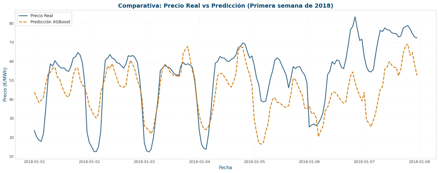
# Prodicciones sobre el conjunto de validación
y_val_pred = xgb_pipeline.predict(X_val)

rmse_val = np.sqrt(mean_squared_error(y_val, y_val_pred))
mae_val = mean_absolute_error(y_val, y_val_pred)
r2_val = r2_score(y_val, y_val_pred)

print("--- Métricas de Rendimiento en Validación ---")
print(f"RMSE (Error cuadrático medio): {rmse_val:.2f} €/MWh")
print(f"MAE (Error absoluto medio):    {mae_val:.2f} €/MWh")
print(f"R² (Coeficiente de determinación): {r2_val:.4f}")
--- Métricas de Rendimiento en Validación --- RMSE (Error cuadrático medio): 5.49 €/MWh MAE (Error absoluto medio): 3.84 €/MWh R² (Coeficiente de determinación): 0.7229
residuos = y_val - y_val_pred

plt.figure(figsize=(10, 5))
plt.scatter(y_val, residuos, alpha=0.3, color=viz.NOBLUE[1])
plt.axhline(0, color=viz.NORANGE[0], linestyle='--')
plt.title('Distribución de residuos (¿El modelo falla más cuando el precio es alto?)')
plt.xlabel('Precio Real')
plt.ylabel('Error (Real - Pred)')
plt.grid(True, alpha=0.3)
plt.tight_layout()
plt.show()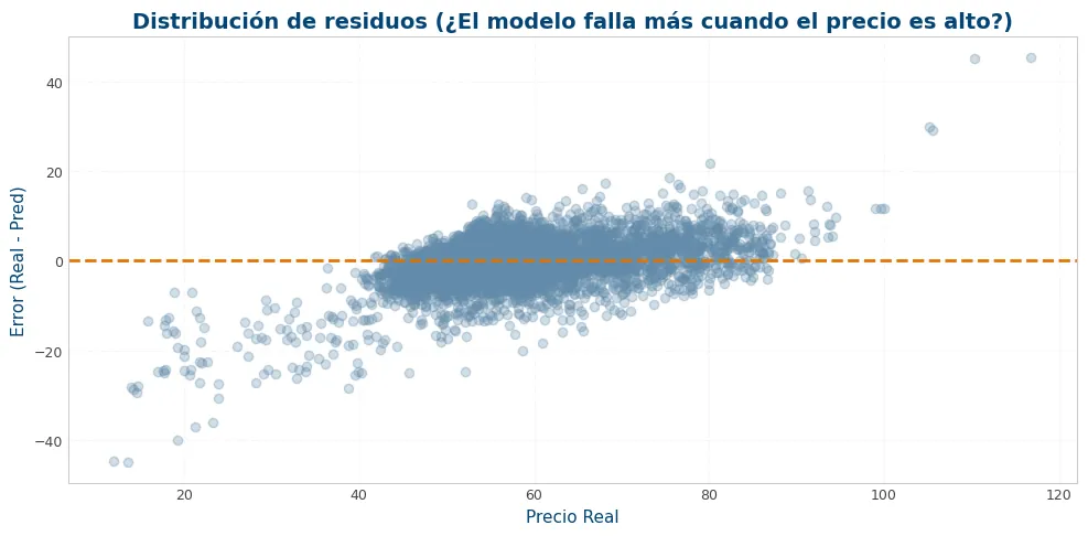
#Evaluación final sobre el conjunto de test aislado (2018)
# (xgb_pipeline ya se cargó en la sección de evaluación; el pipeline escala internamente)
y_final_pred = xgb_pipeline.predict(X_final_test)

rmse_final = np.sqrt(mean_squared_error(y_final_test, y_final_pred))
mae_final = mean_absolute_error(y_final_test, y_final_pred)
r2_final = r2_score(y_final_test, y_final_pred)

print(f"RMSE (Error cuadrático medio): {rmse_final:.2f} €/MWh")
print(f"MAE  (Error absoluto medio):   {mae_final:.2f} €/MWh")
print(f"R²   (Coeficiente de determinación): {r2_final:.4f}")
print(f"\nNº de registros en test: {len(y_final_test)}")

plt.figure(figsize=(16, 6))
plt.plot(y_final_test.index[:720], y_final_test[:720],
         label='Precio Real (€/MWh)', color=viz.NOBLUE[0], linewidth=1.5)
plt.plot(y_final_test.index[:720], y_final_pred[:720],
         label='Predicción XGBoost', color=viz.NORANGE[0], linestyle='--', linewidth=1.5)
plt.title('Evaluación Final: Real vs Predicción — Enero 2018 (Test Aislado)', fontsize=14)
plt.xlabel('Fecha')
plt.ylabel('Precio (€/MWh)')
plt.legend()
plt.grid(True, alpha=0.3)
plt.tight_layout()
plt.show()

residuos_final = y_final_test - y_final_pred

plt.figure(figsize=(14, 5))

plt.subplot(1, 2, 1)
plt.scatter(y_final_test, residuos_final, alpha=0.4, color=viz.NOBLUE[1])
plt.axhline(0, color=viz.NORANGE[0], linestyle='--')
plt.title('Residuos vs Precio Real (Test 2018)')
plt.xlabel('Precio Real (€/MWh)')
plt.ylabel('Residuo (Real - Pred)')

plt.subplot(1, 2, 2)
plt.hist(residuos_final, bins=60, color=viz.NOBLUE[1], edgecolor='white', alpha=0.8)
plt.title('Distribución de Residuos (Test 2018)')
plt.xlabel('Error (€/MWh)')
plt.ylabel('Frecuencia')

plt.tight_layout()
plt.show()

print(f"Error medio (bias): {residuos_final.mean():.3f} €/MWh")
print(f"Error máximo absoluto: {residuos_final.abs().max():.2f} €/MWh")
print(f"Percentil 95 del |error|: {residuos_final.abs().quantile(0.95):.2f} €/MWh")
RMSE (Error cuadrático medio): 6.49 €/MWh MAE (Error absoluto medio): 4.66 €/MWh R² (Coeficiente de determinación): 0.7087 Nº de registros en test: 8735
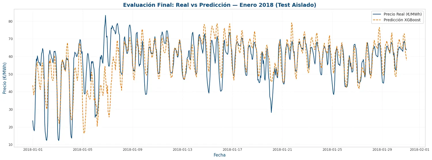
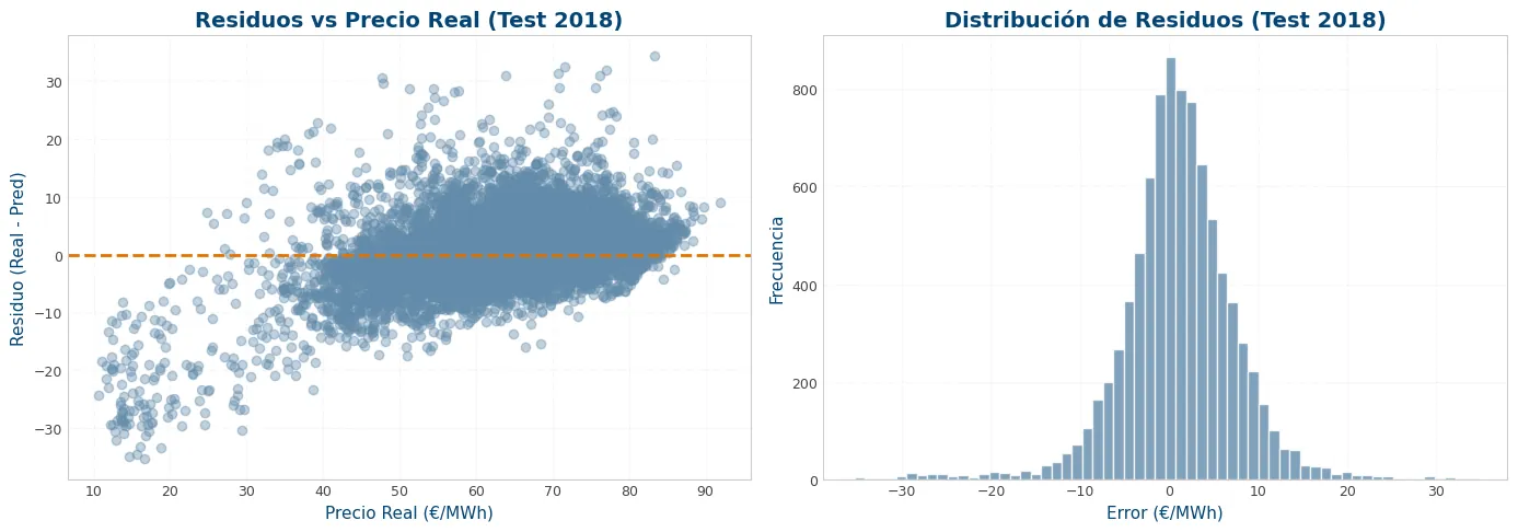
Error medio (bias): 1.011 €/MWh
Error máximo absoluto: 35.32 €/MWh
Percentil 95 del |error|: 12.70 €/MWh
7.1 Importancia de variables (Feature Importance)
¿En qué se apoya el modelo para predecir? Esto justifica el feature engineering realizado.
# Importancia de variables del modelo XGBoost
model = xgb_pipeline.named_steps['regressor']
feat_names = [n.replace('num__', '') for n in xgb_pipeline.named_steps['preprocessor'].get_feature_names_out()]
importancias = pd.Series(model.feature_importances_, index=feat_names).sort_values(ascending=False)

top_n = 20
top = importancias.head(top_n).iloc[::-1]

fig, ax = plt.subplots(figsize=(10, 8))
ax.barh(top.index, top.values, color=viz.NOBLUE[0])
ax.set_title(f'Top {top_n} variables más importantes (XGBoost)')
ax.set_xlabel('Importancia relativa')
plt.tight_layout()
plt.show()

print("Top 10 variables:")
print(importancias.head(10).round(4))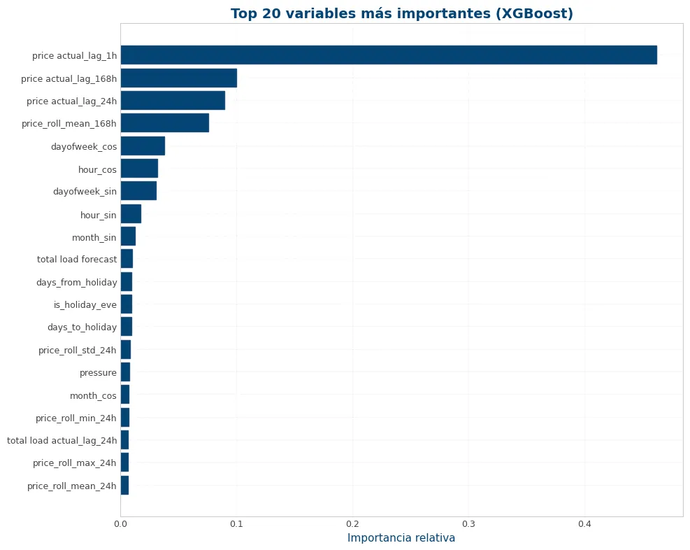
Top 10 variables:
price actual_lag_1h      0.4617
price actual_lag_168h    0.0999
price actual_lag_24h     0.0897
price_roll_mean_168h     0.0755
dayofweek_cos            0.0377
hour_cos                 0.0317
dayofweek_sin            0.0303
hour_sin                 0.0174
month_sin                0.0123
total load forecast      0.0102
dtype: float32
8. Modelo V2:
El modelo base alcanza un R² ≈ 0.72. Intentaremos mejorar la predicción del precio a partir de fundamentales y de autorregresión:
8.1 Reconstrucción de features
Pipeline reproducible y optimizado a partir de lo que se realizó en V1. Ya se descartaron features que no aportaban al modelo dejando solo las útiles y que tienen peso suficiente.
energy_v2 = pd.read_parquet('../data/energy_silver.parquet/')
cols_energia = ['time', 'generation hydro pumped storage consumption',
                'forecast solar day ahead', 'forecast wind onshore day ahead',
                'total load forecast', 'total load actual', 'price actual', 'price day ahead']
energy_v2 = energy_v2[[c for c in cols_energia if c in energy_v2.columns]].copy()

weather_v2 = pd.read_parquet('../data/weather_features_silver.parquet').drop(columns=['weather_description'])
weather_v2['city_name'] = weather_v2['city_name'].str.strip()
weather_v2['peso'] = weather_v2['city_name'].map(pesos_ciudades)

ang = np.radians((90 - weather_v2['wind_deg']) % 360)
weather_v2['wind_x'] = weather_v2['wind_speed'] * np.cos(ang)

# Agregación climática ponderada por ciudad
cols_clima_v2 = ['temp', 'humidity', 'pressure', 'wind_speed', 'wind_x', 'clouds_all', 'rain_1h']

def _pond_v2(g):
    w = g['peso'].values
    return pd.Series({c: np.average(g[c], weights=w) for c in cols_clima_v2})

# include_groups=False evita el FutureWarning de pandas y no mete 'time' en el grupo
weather_nac_v2 = weather_v2.groupby('time').apply(_pond_v2, include_groups=False).reset_index()

# Merge + índice temporal
dfv = pd.merge(weather_nac_v2, energy_v2, on='time', how='outer').sort_values('time').reset_index(drop=True)
dfv['time'] = pd.to_datetime(dfv['time'], utc=True).dt.tz_localize(None)
dfv = dfv.set_index('time')

# Serie horaria continua y ordenada
dfv = dfv.asfreq('h')

# Interpolación SOLO de exógenas; el precio NO se interpola
precio_raw = dfv['price actual'].copy()
exog = [c for c in dfv.select_dtypes(include=[np.number]).columns if c != 'price actual']
dfv[exog] = dfv[exog].interpolate('linear', limit_direction='both')

# festivos + víspera
dfv['is_holiday'] = dfv.index.normalize().isin(festivos_dt).astype(int)
dfv['is_holiday_eve'] = dfv.index.normalize().isin(festivos_dt - pd.Timedelta(days=1)).astype(int)
dfv['weekend'] = (dfv.index.dayofweek >= 5).astype(int)

# Variables cíclicas
for col, periodo in {'hour': 24, 'dayofweek': 7, 'month': 12}.items():
    v = getattr(dfv.index, col)
    dfv[f'{col}_sin'] = np.sin(2 * np.pi * v / periodo)
    dfv[f'{col}_cos'] = np.cos(2 * np.pi * v / periodo)

# Demanda residual prevista
dfv['residual_load'] = dfv['total load forecast'] - dfv['forecast solar day ahead'] - dfv['forecast wind onshore day ahead']
dfv['renew_ratio']   = (dfv['forecast solar day ahead'] + dfv['forecast wind onshore day ahead']) / dfv['total load forecast']

# Es el mínimo limpio (deja 1 h de margen sobre el corte).
GAP = 12
pg = precio_raw.shift(GAP)  # precio más reciente garantizado al cierre de las 12:00

dfv['price_roll_mean_24h']  = pg.rolling(24).mean()
dfv['price_roll_mean_168h'] = pg.rolling(168).mean()
dfv['price_roll_std_24h']   = pg.rolling(24).std()
dfv['price_roll_min_24h']   = pg.rolling(24).min()
dfv['price_roll_max_24h']   = pg.rolling(24).max()

# Lags de precio. shift(k) sobre t = (k + 24) h antes del target.
for lag in [12, 36, 168]:
    dfv[f'price actual_lag_{lag}h'] = precio_raw.shift(lag)

# Predictores alineados t+24
dfv['load_fc_target']  = dfv['total load forecast'].shift(-24)
dfv['solar_fc_target'] = dfv['forecast solar day ahead'].shift(-24)
dfv['wind_fc_target']  = dfv['forecast wind onshore day ahead'].shift(-24)
dfv['resid_fc_target'] = dfv['load_fc_target'] - dfv['solar_fc_target'] - dfv['wind_fc_target']

# Clima (shift -24).
for c in ['temp', 'clouds_all', 'humidity', 'wind_speed', 'wind_x', 'pressure']:
    dfv[f'{c}_target'] = dfv[c].shift(-24)

# Target
dfv['target_price_24h'] = precio_raw.shift(-24)

cols_fuera = ['target_price_24h', 'price actual', 'total load actual',
              'price day ahead', 'pda_target',
              'generation hydro pumped storage consumption',
              'temp', 'humidity', 'pressure', 'wind_speed', 'wind_x',
              'clouds_all', 'rain_1h']

# dropna SOLO sobre lo que el modelo usa (X + target), como dice el comentario
X_cols = [c for c in dfv.columns if c not in cols_fuera]
dfv = dfv.dropna(subset=[*X_cols, 'target_price_24h'])

X_v2 = dfv[X_cols]
y_v2 = dfv['target_price_24h']

print(f"Dataset V2 listo: {dfv.shape} | nº features en X: {X_v2.shape[1]}")
Dataset V2 listo: (33207, 44) | nº features en X: 32
Lo que hemos añadido (V2):
Predictores alineados a la hora objetivo (t+24): las previsiones day-ahead de demanda, solar y eólica, todas publicadas antes del cierre de la subasta de las 12:00 del día anterior, por lo que no introducen fuga de información. Se incluye también el clima del día objetivo; al no disponer de previsiones meteorológicas históricas, se usa la observación real como proxy de la previsión. Esto introduce un ligero sesgo optimista, mayor en viento y nubosidad que en temperatura (más predecible a 24h). El análisis de importancia confirma que estas variables tienen un peso bajo en el modelo, por lo que el efecto del proxy sobre las métricas es marginal.
Demanda residual prevista (carga prevista − solar prevista − eólica prevista), que aproxima la generación que debe cubrir la tecnología marginal y es uno de los principales drivers del precio.
Lags de precio en [12, 36, 168] horas y estadísticos móviles de tendencia (medias a 24h y 168h), volatilidad (desviación a 24h) y extremos (máx/mín a 24h). Todos los lags y ventanas se desplazan de forma que su dato más reciente es anterior al cierre de la subasta para las 24 horas objetivo, respetando la mecánica del mercado y evitando fuga de información.
tr_v2 = dfv.index < cutoff_date
te_v2 = dfv.index >= cutoff_date
X_dev_v2, y_dev_v2 = X_v2[tr_v2], y_v2[tr_v2]
X_test_v2, y_test_v2 = X_v2[te_v2], y_v2[te_v2]

X_tr2, X_val2, y_tr2, y_val2 = train_test_split(
    X_dev_v2, y_dev_v2, test_size=0.2, random_state=42, shuffle=False)

num_feat_v2 = X_tr2.select_dtypes(include=np.number).columns.tolist()
pre_v2 = ColumnTransformer([('num', StandardScaler(), num_feat_v2)])
pre_v2.fit(X_tr2)

xgb_v2 = xgb.XGBRegressor(
    objective='reg:squarederror',
    random_state=32,
    n_estimators=15000,
    early_stopping_rounds=150,
    max_depth=4,
    min_child_weight=5,
    learning_rate=0.003,
    reg_alpha=1.0,
    reg_lambda=1.0,
    subsample=0.8,
    colsample_bytree=0.8,
    tree_method='hist', device='cuda')

print("Entrenando Modelo V2 ...")
xgb_v2.fit(pre_v2.transform(X_tr2), y_tr2,
           eval_set=[(pre_v2.transform(X_val2), y_val2)], verbose=500)
print(f"Árbol óptimo: {xgb_v2.best_iteration}")
Entrenando Modelo V2 ... [0] validation_0-rmse:11.60041 [500] validation_0-rmse:6.93693 [1000] validation_0-rmse:6.08579 [1500] validation_0-rmse:5.79850 [2000] validation_0-rmse:5.67524 [2500] validation_0-rmse:5.61397 [3000] validation_0-rmse:5.56666 [3500] validation_0-rmse:5.52368 [4000] validation_0-rmse:5.48560 [4500] validation_0-rmse:5.45246 [5000] validation_0-rmse:5.42507 [5500] validation_0-rmse:5.40199 [6000] validation_0-rmse:5.38365 [6500] validation_0-rmse:5.36533 [7000] validation_0-rmse:5.35087 [7500] validation_0-rmse:5.33654 [8000] validation_0-rmse:5.32386 [8500] validation_0-rmse:5.31120 [9000] validation_0-rmse:5.30183 [9500] validation_0-rmse:5.29295 [10000] validation_0-rmse:5.28267 [10500] validation_0-rmse:5.27318 [11000] validation_0-rmse:5.26416 [11500] validation_0-rmse:5.25456 [12000] validation_0-rmse:5.24618 [12500] validation_0-rmse:5.24052 [13000] validation_0-rmse:5.23403 [13500] validation_0-rmse:5.22870 [14000] validation_0-rmse:5.22090 [14500] validation_0-rmse:5.21534 [14999] validation_0-rmse:5.20918 Árbol óptimo: 14979
y_pred_v2 = xgb_v2.predict(pre_v2.transform(X_test_v2))
rmse_v2 = np.sqrt(mean_squared_error(y_test_v2, y_pred_v2))
mae_v2 = mean_absolute_error(y_test_v2, y_pred_v2)
r2_v2 = r2_score(y_test_v2, y_pred_v2)

print(f"RMSE: {rmse_v2:.2f} €/MWh  |  MAE: {mae_v2:.2f} €/MWh  |  R²: {r2_v2:.4f}")
print(f"(Modelo base V1 era R² ≈ 0.72)")

# Comparativa real vs predicción (primer mes de 2018)
plt.figure(figsize=(16, 6))
plt.plot(y_test_v2.index[:720], y_test_v2[:720], label='Precio Real',
         color=viz.NOBLUE[0], linewidth=1.5)
plt.plot(y_test_v2.index[:720], y_pred_v2[:720], label='Predicción V2 (purista)',
         color=viz.NORANGE[0], linestyle='--', linewidth=1.5)
plt.title(f'Modelo V2 purista: Real vs Predicción — Enero 2018  (R²={r2_v2:.3f})', fontsize=14)
plt.xlabel('Fecha')
plt.ylabel('Precio (€/MWh)')
plt.legend()
plt.grid(True, alpha=0.3)
plt.tight_layout()
plt.show()
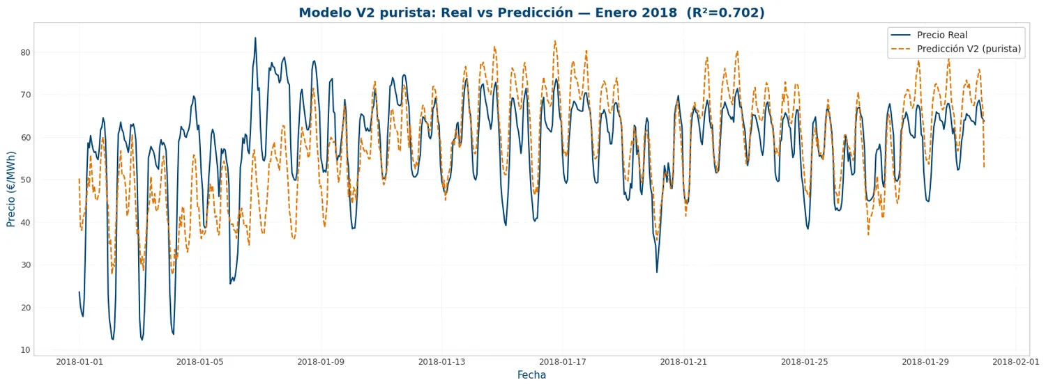
RMSE: 6.61 €/MWh | MAE: 4.95 €/MWh | R²: 0.7016 (Modelo base V1 era R² ≈ 0.72)
feat_v2 = [n.replace('num__', '') for n in pre_v2.get_feature_names_out()]
imp_v2 = pd.Series(xgb_v2.feature_importances_, index=feat_v2).sort_values(ascending=False)

top = imp_v2.head(20).iloc[::-1]
fig, ax = plt.subplots(figsize=(10, 8))
ax.barh(top.index, top.values, color=viz.NOBLUE[0])
ax.set_title('Top 20 variables más importantes — Modelo V2 (purista)')
ax.set_xlabel('Importancia relativa')
plt.tight_layout()
plt.show()

print("Top 10 variables (V2):")
print(imp_v2.head(10).round(4))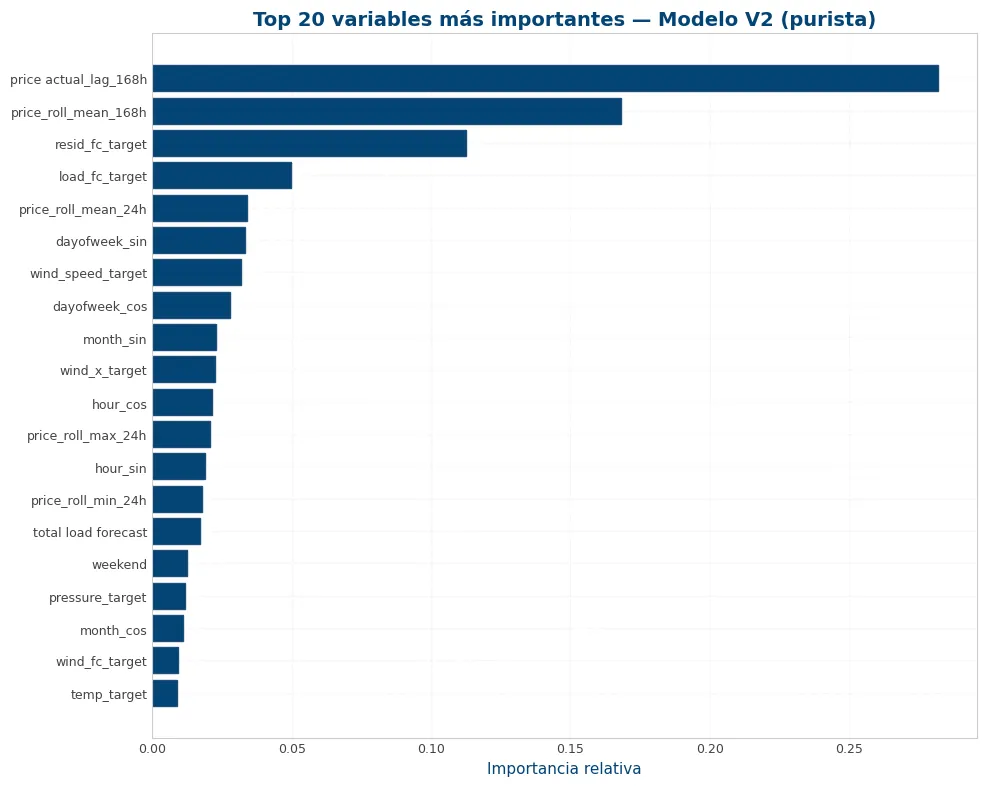
Top 10 variables (V2):
price actual_lag_168h    0.2817
price_roll_mean_168h     0.1680
resid_fc_target          0.1124
load_fc_target           0.0499
price_roll_mean_24h      0.0338
dayofweek_sin            0.0334
wind_speed_target        0.0320
dayofweek_cos            0.0280
month_sin                0.0229
wind_x_target            0.0224
dtype: float32
9. Conclusiones
Mi objeto era crear un modelo robusto con las técnicas que conocía + ir aprendiendo durante el proceso. El modelo XGBoost explica en torno al 70% de la variabilidad del precio en el test aislado de 2018. Tras corregir los data leaks, el V2 con fundamentales day-ahead se queda a la par del V1 autorregresivo: los lags de precio ya capturaban casi toda la señal aprovechable. No he podido conseguir más debido a que españa cuenta con uno de los sistemas eléctricos mas impredecibles del mundo.
El modelo es más débil frente a los picos de demanda y en el contexto de españa se situaba en plena transición energética dificultando tadavía más realizar las predicciones de cara a 2018.
En el futuro sería ideal tener variables externas como el impuesto al CO2 y también tener datasets más recientes.
Actualización Encontré un par de data leaks de los que no me di cuenta por estar haciendo unas pruebas. Actualmente los lags y rollings solo se crean con horas legítimas para el modelo.